A high tidal figure fails as a comparison until you name its denominator. Conversion efficiency, the power coefficient, annual capacity factor and predictability use different denominators, units, time scales and boundaries.
Tidal power has no single efficiency in the two primary documents behind this page. The U.S. Department of Energy’s April 2019 glossary defines conversion efficiency as energy turned into a useful form, such as electricity, divided by the total energy available to the device, and it defines capacity factor as mean generation divided by peak generation over a reference period. The 2009 EMEC performance guide, first published by BSI, defines the power coefficient as electrical power divided by the kinetic power in a stream tube the size of the capture area. Annual energy in that guide is a separate product: a measured power curve, a year of predicted current speeds, and a stated availability. Predictability sits with the forecast. Engineering LibreTexts, retrieved 11 October 2026, prints one plant pair that shows the split: the Rance barrage, maximum power 240 MW, average power 57 MW, a capacity factor of about 24%. That pair is mean against peak for one barrage.
Ocean Energy Notes compiled the table and the reading path from those documents. How a tidal stream differs from a tidal range, including slack water, is already set out in wave energy versus tidal energy.
Key points
- Name the denominator before you compare two tidal percentages.
- Conversion efficiency, in the April 2019 glossary, uses the energy available to the device.
- The power coefficient, in the 2009 guide, uses the kinetic power across the capture area. The guide does not print a plant value for it.
- Capacity factor, in the same glossary, uses peak generation over a stated period, or the same idea in full-load hours per year.
- A predicted tide is an input to annual energy. It is a separate column from the three ratios.
What does a tidal efficiency percentage measure?
It measures whichever ratio the writer actually divided. The April 2019 glossary and the 2009 guide use the labels below. A percentage that arrives without its row is not yet a result you can compare.
| Quantity | Denominator | Unit | Time scale | Boundary |
|---|---|---|---|---|
| Device conversion efficiency | Total energy available to the device. The glossary does not define that available energy any further. | A proportion. The entry does not say to multiply by 100. | The glossary does not set the window. | One device. Useful form in the example is electricity. |
| Power coefficient | Kinetic power in a stream tube with the same capture area as the rotor. Equation 4 writes electrical power over ½ ρ A U³. | A ratio. The guide does not say to print it as a percent. | Simultaneous with the recorded power and the performance velocity. | A tidal energy conversion system in a free stream. Electrical power, after the drive train. Varies with tip speed ratio. |
| Annual capacity factor | Peak generation on that generator. The glossary also allows equivalent full-load hours per year. | A percentage for a reference period, or hours per year. | The reference period the report names. “Annual” still needs that period in print. | Mean generation against peak generation. Installed capacity is a separate glossary entry, in kW or MW, and the capacity-factor entry does not tell you to substitute it. |
| Predictability | None. It is not an output divided by an energy input. | A forecast of tidal current, then used inside the annual-energy product. | One year, in the guide’s definition of estimated annual energy production. | The forecast feeds the calculation. It does not replace the measured power curve or the stated availability. |
| Availability, EMEC wording | Hours in the specified period. Subtract hours the device could not run because of maintenance or a fault. | A percentage. | The specified period. | Logged apart from grid faults and other third-party stops. The guide says lack of electric output is not itself the availability signal. |
The Department of Energy defines availability in the same glossary as the percentage of time a device is operational and able to convert energy. That sentence and the EMEC sentence are both percentages of time. They are still different from capacity factor, which compares mean generation with peak generation.

The photograph shows an instrument on a line. It is not a record from a named trial, and it is not a Grays Harbor installation. Clause 5.2 of the 2009 guide asks for a device that records horizontal current velocity and direction through the water column, specified to measure velocity to ±2% or better and verified by traceable calibration. The ±2% is an instrument bound on the velocity reading. It is not a tidal-plant efficiency.
Takeaway: Put the percentage in a row before you repeat it. If the denominator cell is empty, the number is not ready to compare.
How do you get from an EMEC power curve to annual energy?
You keep six records from the 2009 guide in order, and you stop when a record is missing. The guide says its information is for guidance and is not a substitute for technical advice in a specific situation. This page uses it as a reading path. It does not claim the 2009 text is the current mandatory test standard.
-
Run the device in normal operation for at least 15 days, or longer if the curve has not converged. Leave the configuration and the control algorithm unchanged. The guide asks for intermediate curves from each successive 24 hours of valid operation, and it says an uninterrupted day adds 144 readings.
-
Build one performance velocity for each record. Slice the capture area at 1 m or finer, from the seabed up. For a fixed device, use only the velocity component perpendicular to the capture surface. For a device that turns into the current, use the velocity vector. Equation 2 combines those slices into U_perf. The current records are at about 10 minutes, time-stamped to UTC.
-
Bin that velocity in steps of 0.10 m/s. The guide prints the step as 0,10 m/s. In each bin, average the performance velocity and average the electrical power. Power for the curve is the power at the device output, so drive-train losses stay inside it. If the meter is at an onshore substation instead, the guide says to account for cables, transformers and power conditioning.
-
If a power-coefficient curve was agreed at the start, divide that electrical power by the kinetic power ½ ρ A U_perf³. Where freshwater input is insignificant, the guide allows a representative seawater density of 1,025 kg/m³, printed there as 1 025 kg/m³. Where density would vary, it asks for temperature and salinity beside the current meter. The coefficient is a function of tip speed ratio, the rotor tip speed divided by the free-stream speed. The guide says performance is likely to fall below the theoretical Betz limit for an infinite stream, and that the seabed and free surface can let a device reach or exceed that limit. It does not print a percentage for the limit.
-
Remove periods when the device was unavailable from the power calculation, and still report availability for the test period. Log maintenance and faults on the device. Log grid faults and other third-party stops on their own lines. Clause 5.4 says non-production of electric power is not a suitable availability signal, and it gives a grid failure as the example.
-
Estimate annual energy production in kilowatt-hours with equation 5: multiply 8760 by the predicted availability, then by the sum over bins of bin power in kilowatts times the fraction of the year spent in that bin. The factor 8760 equals 365 days times 24 hours, so a power in kilowatts times a fraction of a non-leap year becomes kilowatt-hours. Quote the result with a margin from the bin uncertainties. Another site needs that site’s own fractions of time at each velocity. The guide says those uncertainties cover the performance test, and that a practical forecast also has to account for availability lost to storm damage and other influences.
The definition expresses availability as a percentage. Equation 5 multiplies by the predicted availability. The guide does not print a worked number that shows whether that factor enters as 0.95 or as 95. Read the unit in the test report before you multiply.
Moving water is the resource on the horizontal axis of the power curve. The photograph is a generic channel. It is not a measured velocity series, and the streaks are not a power curve.
Takeaway: Annual energy is the curve times a year of predicted speeds, times a stated availability. A single percentage does not store that product.
Where do the published percentages sit?
They sit in different rows. The figures below are copied from pages retrieved on 11 October 2026. This article does not remeasure the plants, and it does not fill a denominator the page left blank.
| Figure as printed | Page | Denominator on that page | Time scale on that page | Boundary |
|---|---|---|---|---|
| about 24% | Engineering LibreTexts, on the Rance Tidal Power Station | Average power 57 MW divided by maximum power 240 MW. 57 ÷ 240 = 0.2375, which is the ratio behind the printed “about 24%.” | The page does not state the years inside the average. | One barrage in the La Rance estuary, operating since 1966, at a tidal range the page describes as high as 8 meters. Under the April 2019 glossary this shape is a capacity factor. The paragraph does not give a conversion efficiency or a power coefficient. |
| around 80% | Ormazabal, “the capacity factor of such facilities” | The page does not state a mean output or a peak. | The page does not state a year or a period. | No plant is named. The same page says effective power generation is limited to a maximum of 10 hours per day, and it does not show a calculation that connects those 10 hours to the 80%. |
| about 20% | Engineering LibreTexts, citing an Encyclopedia Britannica article | Global power consumption, in the page’s wording. The power it compares is an estimate of 3,000 GW contained in tides worldwide. | The page does not attach the 20% to a year of plant output. | A worldwide resource comparison. This page did not reopen the Britannica article. The 20% is not a device conversion efficiency. |
The 0.2375 figure is arithmetic on the two powers LibreTexts prints. It is not a new measurement. The same LibreTexts page describes a barrage cycle with two generating sessions and two pauses in half a day. That pause structure is why a capacity factor for a barrage can sit far from continuous full output. It still does not identify the years inside the 57 MW average.
The Ormazabal 80% is the kind of high number that starts this page. The words “capacity factor” are on the page. The mean, the peak, the plant and the year are not. Those empty cells are the result. This page does not adopt 80% as a typical tidal value, and it does not turn “10 hours per day” into a percentage of its own.
Where does predictability sit?
It sits upstream of annual energy, as a forecast of the current. Clause 3.1.5 defines estimated annual energy production as the total energy production of a device during one year, obtained by applying the measured power curve to a set of tidal current predictions, at a stated availability. The curve is a measurement. The current predictions are the predictable part. Availability is the third factor in the product.
Equation 1 writes the kinetic power across the capture area as ½ ρ A U_perf³. When the performance velocity is small, that kinetic power is small because the velocity is cubed. A forecast that includes slow water still assigns those hours the power the curve gives for that bin. Predictable timing does not fill a slow bin with the power from a fast bin.
The April 2019 glossary defines an intermittent energy source as one that is not continuously available for conversion into electricity and is outside direct control because the primary energy cannot be stored. It defines variable generation as nondispatchable because the resource fluctuates. Those two entries leave room for a tide you can time and an output that still changes through the cycle. Slack water, when the flow speed drops to zero, is separated from predictability on wave energy versus tidal energy.
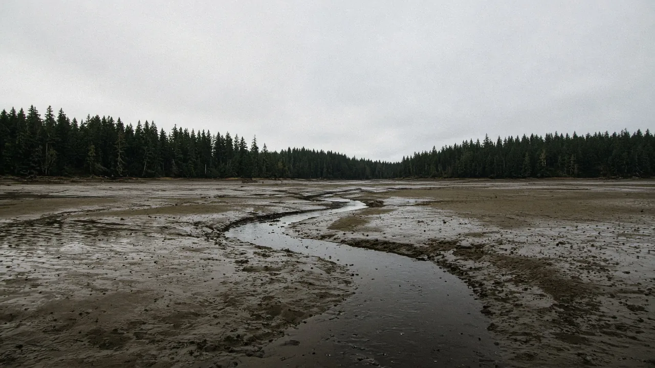
Low water on a temperate estuary. The photograph shows a resource that has changed with the tide. It is not a generation record, and it is not a project site.
Takeaway: Ask whether the sentence forecasts the current, or whether it divides output by an energy input. Only the second kind belongs in the efficiency rows.
When this reading does not apply
The path above is for a free-stream device with a measured curve of electrical power against current velocity. Use a different record when the machine is not that.
- A barrage or a tidal-range plant. The EMEC power coefficient uses a stream tube and a capture area. A barrage uses a difference in water level. The Rance 24% can be read as mean power over maximum power. It cannot be read as that power coefficient.
- A universal tidal efficiency. The documents opened for this page do not print one, and this page does not supply one. There is no side-by-side set of current device tests here.
- A nameplate shortcut. The glossary’s capacity factor uses peak generation, or full-load hours. Its installed-capacity entry is the power at full output, traditionally the generator rating, in kilowatts or megawatts. A report that divides annual energy by nameplate times the 8760 in equation 5 is using a denominator it has to state itself.
- Price or a permit. Those questions use other documents. Nothing on this page is a forecast of revenue or a ranking of devices.
- An environmental effect. Barrage and turbine evidence, and the scale each source covers, is set out in tidal energy environmental effects.
The About page states what this independent publication is, and the separation from the former domain holder and from project developers.
Methods and sources
The denominator table uses the April 2019 Department of Energy glossary for conversion efficiency, capacity factor, availability, installed capacity, intermittent energy and variable generation. The reading path uses the 2009 EMEC guide, clauses 3.1.2, 3.1.5, 3.1.10, 5.2, 5.4, 6.2, 7.2, 7.3 and 7.4, including equations 1, 2, 4 and 5. The guide was first published in the UK in 2009 by BSI and is marked as guidance. The worked percentages come from the Engineering LibreTexts page and the Ormazabal page, both retrieved on 11 October 2026. The ratio 0.2375 is 57 divided by 240, the two Rance powers printed on the LibreTexts page. No velocity series was reprocessed, and no device was tested for this article. The photographs are generic scenes.
Full links are in the references below.